Temporal Focusing Microscope
Temporal focusing microscopy is an interesting variation on confocal microscopy where the the excitation beam is spread out not only spatially (as for confocal microscopy) but also temporally, by using diffraction grating to disperse a broadband laser beam. Typically, the method uses the exitation beam to generate 2-photon luminesence in the target which is collected by a large-area detector. The image is formed by raster scanning the exitation focus.
This method makes a nice example of using a diffraction grating in Raypier, and a demonstration of using a BroadbandGaussletSource to model the propagation of a femtosecond ultra-fast pulse.
In this example, we leave out the raster-scanning system (which is relatively uninteresting) so we can focus (no pun intended) on the temporal aspect.
Here’s our model:
from pathlib import Path

from traits.api import Range, Float, observe
from traitsui.api import View, Item, VGroup

from raypier.beamsplitters import UnpolarisingBeamsplitterCube
from raypier.lenses import PlanoConvexLens
from raypier.diffraction_gratings import RectangularGrating
from raypier.gausslet_sources import BroadbandGaussletSource, SingleGaussletSource
from raypier.tracer import RayTraceModel
from raypier.fields import EFieldPlane
from raypier.intensity_image import IntensityImageView
from raypier.intensity_surface import IntensitySurface
from raypier.probes import GaussletCapturePlane
from raypier.constraints import Constraint
from raypier.editors import NumEditor
from raypier.shapes import CircleShape
from raypier.general_optic import GeneralLens
from raypier.faces import AsphericFace, SphericalFace
from raypier.materials import OpticalMaterial


src = BroadbandGaussletSource(
    origin = (0,0,0),
    direction=(1.0,0.0,0.0),
    E_vector=(0,0,1),
    working_dist=0.0,
    number=200,
    wavelength = 1.0,
    wavelength_extent = 0.03,
    bandwidth_nm = 13.0,
    beam_waist = 1000.0,
    display='wires',
    show_paras=False
    )

# src = SingleGaussletSource(
#     origin = (0,0,0),
#     direction=(1.,0.,0.0),
#     working_dist=0.0,
#     wavelength=0.8,
#     beam_waist=1.0, #in microns
#     E_vector=(0,0,1)
#     )

grating = RectangularGrating(centre=(220.0,0.,0.),
                             direction=(-1,1,0.),
                             length=15.,
                             width=20.0,
                             thickness=3.0,
                             lines_per_mm=1400.0)
grating.orientation = 45.5

lens1 = PlanoConvexLens(centre=(40.0,0.0,0.0),
                        direction=(-1,0,0),
                        diameter=25.0,
                        CT=6.0,
                        n_inside=1.6,
                        curvature=100.0)

### Not used now. Use Aspheric instead.
lens2 = PlanoConvexLens(centre=(10.0,-30.0,0.0),
                        direction=(0,1,0),
                        diameter=25.0,
                        CT=6.0,
                        n_inside=1.6,
                        curvature=25.0)

### Construct an aspheric objective using General Lens framework.
### This is intended to represent Edmund Optics #66-330
circle = CircleShape(radius=10.0)
s1 = AsphericFace(z_height=0.0,
                  curvature=1./8.107287E-02,
                  conic_const=-6.196140E-01,
                  A6=-1.292772E-08, #I'm not 100% sure if the signs of the polynomial terms are right.
                  A8=-1.932447E-10
                  )
s2 = SphericalFace(curvature=-200.0,
                   z_height=-8.0)
mat = OpticalMaterial(glass_name="L-BAL35")
asphere = GeneralLens(name="Sample Objective",
                      centre=(10.0,-30.0,0.0),
                      direction=(0,1,0),
                      shape=circle,
                      surfaces=[s2,s1],
                      materials=[mat])

bs = UnpolarisingBeamsplitterCube(centre = (10.0, 0., 0.),
                                  size=15.0,
                                  )

capture = GaussletCapturePlane(centre=(10,-53.3,0),
                               direction=(0,1,0),
                               width=15.0,
                               height=15.0)

field = EFieldPlane(centre=(10,-53.3,0),
                    direction=(0,0,1),
                    detector=capture,
                    align_detector=True,
                    size=100,
                    width=0.1,
                    height=0.5,
                    time_ps=-7.0)

image = IntensityImageView(field_probe=field)
surf = IntensitySurface(field_probe=field)


class MyConstraint(Constraint):
    time = Range(-15.0,15.0,-7.0)
    time_offset = Float(0.0)

    traits_view = View(VGroup(
        Item("time", style='custom'),
        Item("time_offset", editor=NumEditor)
        ))

    @observe("time, time_offset")
    def on_time_change(self, evt):
        field.time_ps = self.time + self.time_offset


    def animate(self, dt, count):
        for i in range(count):
            field.time_ps = self.time + self.time_offset + i*dt
            U = field.intensity
            image.save_plot(f"{Path.home()}/range_{i:03d}.png")

cst = MyConstraint()

model = RayTraceModel(optics = [bs, grating, lens1, asphere],
                      sources = [src], probes=[field, capture],
                      results=[image,surf],
                      constraints = [cst])

model.configure_traits()
The BroadbandGaussletSource creates a set of Gausslets with centre wavelength of 1.0 micron, and covering a total wavelength range of 0.03 micron (i.e. 30nm). Thus the wavelengths cover the range from 0.85 micron to 1.15 micron. We choose to create 200 Gausslets over this range. The E-field amplitudes of theses Gausslets has a Gaussian profile centered on the centre-wavelength. This bandwidth is set to be 13nm. The Gausslets will actually be uniformly spaced in frequency and will thus necessarily be non-uniformly spaced in terms of wavelength.
Since a single monochromatic Gausslet represents a periodic E-field amplitude (i.e. a sine-wave), a linear combination of a finite set of such Gausslets is also periodic. It turns out our source creates a periodic pulse train where the interval between pulses is given by the inverse of the frequency-spacing of the Gausslets. If you want very widely spaced pulses, you thus need a smaller frequency-spacing and hence a larger number of rays. To keep the calculation times reasonable, it’s best to use the shortest pulse-separation you can get away with to achieve your model objectives.
The 3D view of the model looks like this:
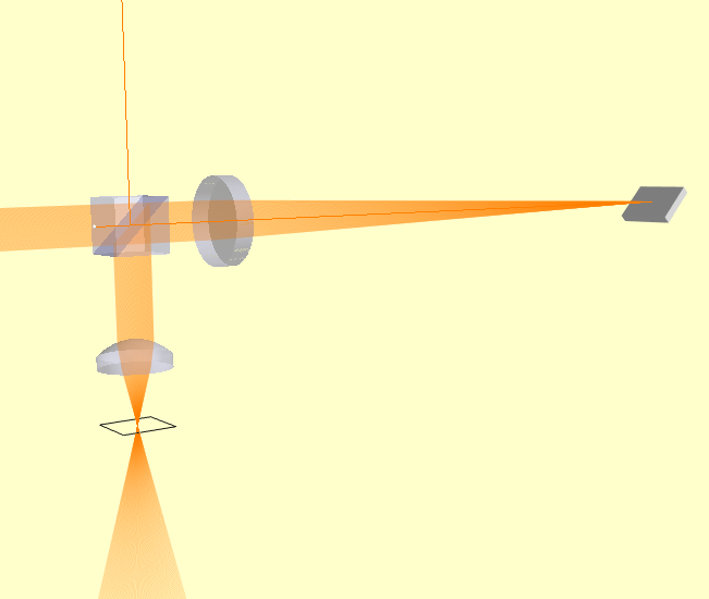
The beam is lauched on the left side of this view and is propagated through the beam-splitter cube (the reflected beam travelling upwards is discarded). The beam passes through a spherical lens with 200mm focal length. This focuses the beam onto a diffraction grating. The grating disperses the beam into its 1st order of difraction and we can see the lateral spread of the beam as it propagates back to the beam-splitter. The reflected beam from the beam-splitter passes through a aspheric objective lens and comes to a focus. The intersting characteristic here is that when the dispersed beams come into focus they also arrive back in phase, maximising the intensity at the focus.
The intensity profile of the beam is shown in the IntensityImageView object. The EFieldPlane object have a time trait which defines the time at which the E-field is computed by advancing the phase of each wavelength accordingly. The time value of 0.0 will correspond to a pulse centered at the origin of the source object. However, the periodic nature of the beam means that the pulse can be found at repetitions of the pulse-interval along the beam-path. We have created a Constraint object for this example simplify manual adjustment of the observation time-value and for the creation of animations of a field-profile.
Here’s the animation of the pulse intensity from t=-9ps to -5ps:
The vertical axis of the image corresponds to the optical axis (the Y-axis) of the model at the object plane. Yes, the pulse-envelop really does appear to move sideways (orthonally to the beam axis). Note, however, that the image colour scale is always “auto-scaled” which can be deceiving.