Michelson Interferometer

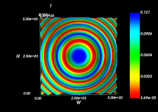
We can create a Michelson interferometer from a non-polarising beam-splitter and two mirrors. The second mirror has a spherical surface to generate a spherical wavefront at the detector-plane. The intensity distribution shows the classic Newton’s Rings type pattern.

from raypier.api import RayTraceModel, UnpolarisingBeamsplitterCube, CollimatedGaussletSource, CircleShape, GeneralLens,\
        SphericalFace, PlanarFace, OpticalMaterial, PolarisingBeamsplitterCube, ParallelRaySource,\
        GaussletCapturePlane, EFieldPlane, IntensitySurface
from raypier.intensity_image import IntensityImageView
        
        

src=CollimatedGaussletSource(origin=(-30,0,0),
                             direction=(1,0,0),
                             radius=5.0,
                             beam_waist=10.0,
                             resolution=10.0,
                             E_vector=(0,1,0),
                             wavelength=1.0,
                             display="wires",
                             opacity=0.05,
                             max_ray_len=50.0)
        
        
bs = UnpolarisingBeamsplitterCube(centre=(0,0,0),
                                  size=10.0)

shape = CircleShape(radius=10.0)

f1 = PlanarFace(mirror=True)
f2 = SphericalFace(curvature=2000.0, mirror=True)

m1 = GeneralLens(name="Mirror 1",
                 shape=shape,
                 surfaces=[f1],
                 centre=(0,20,0),
                 direction=(0,-1,0))

m2 = GeneralLens(name="Mirror 2",
                 shape=shape,
                 surfaces=[f2],
                 centre=(20,0,0),
                 direction=(-1,0,0))

cap = GaussletCapturePlane(centre=(0,-20,0),
                           direction=(0,1,0))

field = EFieldPlane(centre=(0,-20,0),
                    direction=(0,1,0),
                    detector=cap,
                    align_detector=True,
                    width=5.0,
                    height=5.0,
                    size=100)

image = IntensityImageView(field_probe=field)
surf = IntensitySurface(field_probe=field)


model = RayTraceModel(optics=[bs, m1, m2],
                      sources=[src],
                      probes=[field, cap],
                      results=[image, surf])

model.configure_traits()

The rendered model looks as follows:

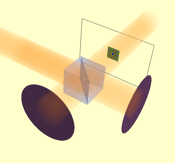
In this case, the E-field evaluation plane is large enough that we can see the intensity profile directly in the model. However, viewing it in a IntensitySurfaceView is more convenient.