Simulating a Bessel Beam

A Pseudo-bessel beam can be created using an Axicon. Where the rays from opposing sides of the axicon interact, they create a region of high intensity along the axis of the axicon. The interested properties of this beam is that it does not diffract. Modelling this with Raypier is straightforward. We use a CollimatedGaussianBeamSource to create the input wavefront.

from raypier.api import GeneralLens, AxiconFace, PlanarFace, OpticalMaterial, CircleShape,\
            RayTraceModel, CollimatedGaussletSource, EFieldPlane, GaussletCapturePlane, IntensitySurface
            
from raypier.intensity_image import IntensityImageView


shape = CircleShape(radius=2.0)

face1 = PlanarFace(z_height=0.0)
face2 = AxiconFace(z_height=1.0, gradient=0.1)

mat = OpticalMaterial(glass_name="N-BK7")

axicon = GeneralLens(name = "My Axicon",
                     centre = (0,0,0),
                     direction=(0,0,1),
                     shape=shape, 
                     surfaces=[face1, 
                               face2], 
                     materials=[mat])

src = CollimatedGaussletSource(origin=(0.001,0,-5.0),
                               direction=(0,0,1),
                               wavelength=0.5,
                               radius=1.0,
                               beam_waist=10.0,
                               resolution=10,
                               max_ray_len=50.0,
                               display='wires',
                               opacity=0.2
                               )

###Add some sensors
capture = GaussletCapturePlane(centre=(0,0,13), 
                               direction=(0,0,1),
                               width=5.0,
                               height=5.0)

field = EFieldPlane(centre=(0,0,13),
                    direction=(0,0,1),
                    detector=capture,
                    align_detector=True,
                    size=100,
                    width=2,
                    height=2)

image = IntensityImageView(field_probe=field)
surf = IntensitySurface(field_probe=field)


model = RayTraceModel(optics=[axicon], 
                      sources=[src], 
                      probes=[capture,field],
                      results=[image,surf])
model.configure_traits()

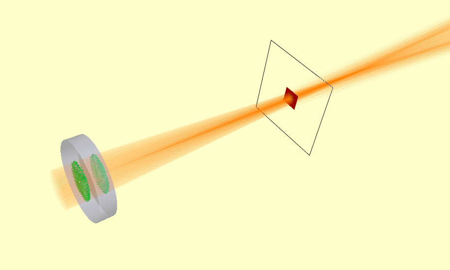
Here’s the model view.

To get accurate results, turn up the resolution of the source object to about 30-40. Reduce the width of the EFieldPanel to ~0.1 to see the centre of the beam more clearly.

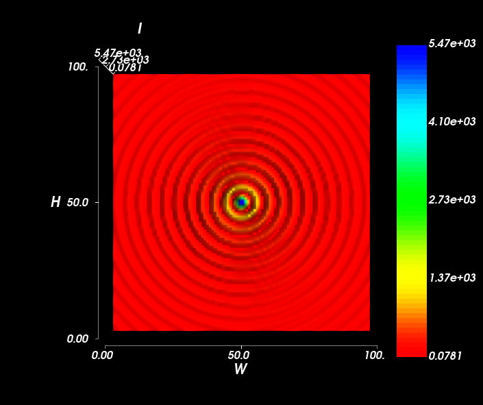
In the XY-plane, the characteristic Bessel rings are clear.

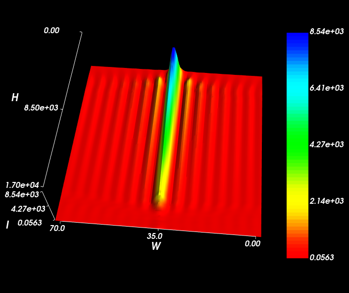
Looking along the Z-axis (the optical axis), the constant width of the central beam is observed.