Distortions
The raypier.distortions module contains objects representing distortions of a given face. The Distortion objects
are intended to be used with the raypier.faces.DistortionFace class (part of the General Optic framework).
Fundamentally, any 2D function can be implemented as a Distortion. At present, on a single type is implemented. I intend
to implement a general Zernike polynomial distortion class. Other distortion functions are easy to add.
An example of their usage:
from raypier.tracer import RayTraceModel
from raypier.shapes import CircleShape
from raypier.faces import DistortionFace, PlanarFace, SphericalFace
from raypier.general_optic import GeneralLens
from raypier.materials import OpticalMaterial
from raypier.distortions import SimpleTestZernikeJ7, NullDistortion
from raypier.gausslet_sources import CollimatedGaussletSource
from raypier.fields import EFieldPlane
from raypier.probes import GaussletCapturePlane
from raypier.intensity_image import IntensityImageView
from raypier.intensity_surface import IntensitySurface

shape = CircleShape(radius=10.0)
f1 = SphericalFace(z_height=0.0, curvature=-25.0)
f2 = PlanarFace(z_height=5.0)

dist = SimpleTestZernikeJ7(unit_radius=10.0, amplitude=0.01)
#dist = NullDistortion()
f1 = DistortionFace(base_face=f1, distortion=dist)

mat = OpticalMaterial(glass_name="N-BK7")
lens = GeneralLens(shape=shape, surfaces=[f1,f2], materials=[mat])

src = CollimatedGaussletSource(radius=8.0, resolution=6,
                               origin=(0,0,-15), direction=(0,0,1),
                               display="wires", opacity=0.2, show_normals=True)
src.max_ray_len=50.0


cap = GaussletCapturePlane(centre = (0,0,50),
                           direction= (0,0,1),
                           width=20,
                           height=20)

field = EFieldPlane(detector=cap,
                    align_detector=True,
                    size=100,
                    width=1,
                    height=1)

img = IntensityImageView(field_probe=field)
surf = IntensitySurface(field_probe=field)


model = RayTraceModel(optics=[lens], sources=[src], probes=[field,cap],
                      results=[img,surf])
model.configure_traits()
This example shows a high-amplitude distortion, for illustrative purposes.
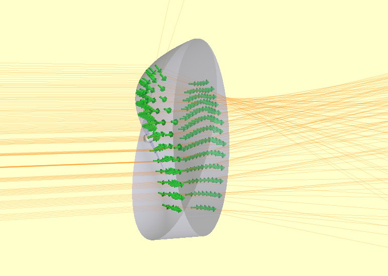
During the ray-tracing operation, the intersections with distorted faces are found using an iterative algorithm similar to Newton- Ralphson. Typically, the intersection is found with 2 to 3 calls to the intercept-method of the underlying face. Distortions are expected to be small deviations from the underlying face (maybe no more than a few wavelengths at most). If you make the amplitude of the distortion large, the under of iterations to converge will increase and the ray-tracing hit take a performance hit. For very large distortions, the intercept my fail altogether.
One could, in principle, wrap multiple DistortionFaces over other DistortionFaces. However, I would expect the performance penalty to be quite severe. In this case, A better plan would be to implement a specialised DistortionList object which can sum the distortion-values from a list of input Distortions. On my todo list …
In python scripting, one can simply evaluate any Distortion object given some x- and y-coordinates as numpy arrays. This is useful for testing. For example:
from raypier.distortions import SimpleTestZernikeJ7
import numpy

dist = SimpleTestZernikeJ7(unit_radius=10.0, amplitude=0,1)

x=y=nmupy.linspace(-10,10,500)
X,Y = numpy.meshgrid(x,y)

Z = dist.z_offset(X.ravel(),Y.ravel())
Z.shape = X.shape #restore the 2D shape of the Z array
Distortions have an additional method, Distortion.z_offset_and_gradient(). This returns a array of shape (N,3)
where the input X and Y arrays have length N. The first two columns of this array contain the gradient of the
distortion, dZ/dX and dZ/dY respectively. The third column simply contains Z. Returning both Z and it’s gradient
turns out to be useful at the C-level during tracing. I.e.:
grad = dist.z_offset_and_gradient(X.ravel(), Y.ravel()).reshape(X.shape[0], X.shape[1],3)
dZdX = grad[...,0]
dZdY = grad[...,1]
Z = grad[...,2]
Zernike Polymonial Distortions
More general distortions can be applied using the raypier.distortions.ZernikeSeries class.
As previously, instances of this object are passed to a raypier.faces.DistortionFace , along
with the base-surface to which the distortion is to be applied.
An example of the this class in action can be seen here:
from raypier.tracer import RayTraceModel
from raypier.shapes import CircleShape
from raypier.faces import DistortionFace, PlanarFace, SphericalFace
from raypier.general_optic import GeneralLens
from raypier.materials import OpticalMaterial
from raypier.distortions import SimpleTestZernikeJ7, NullDistortion, ZernikeSeries
from raypier.gausslet_sources import CollimatedGaussletSource
from raypier.fields import EFieldPlane
from raypier.probes import GaussletCapturePlane
from raypier.intensity_image import IntensityImageView
from raypier.intensity_surface import IntensitySurface
from raypier.api import Constraint

from traits.api import Range, observe
from traitsui.api import View, Item, VGroup


shape = CircleShape(radius=10.0)

#f1 = SphericalFace(z_height=0.0, curvature=-25.0)

f1 = PlanarFace(z_height=0.0)
f2 = PlanarFace(z_height=5.0)

dist = ZernikeSeries(unit_radius=10.0, coefficients=[(i,0.0) for i in range(12)])
f1 = DistortionFace(base_face=f1, distortion=dist)


class Sliders(Constraint):
    """Make a Constrain object just to give us a more convenient UI for adjusting Zernike coefficients.
    """
    J0 = Range(-1.0,1.0,0.0)
    J1 = Range(-1.0,1.0,0.0)
    J2 = Range(-1.0,1.0,0.0)
    J3 = Range(-1.0,1.0,0.0)
    J4 = Range(-1.0,1.0,0.0)
    J5 = Range(-1.0,1.0,0.0)
    J6 = Range(-1.0,1.0,0.0)
    J7 = Range(-1.0,1.0,0.0)
    J8 = Range(-1.0,1.0,0.0)

    traits_view = View(VGroup(
            Item("J0", style="custom"),
            Item("J1", style="custom"),
            Item("J2", style="custom"),
            Item("J3", style="custom"),
            Item("J4", style="custom"),
            Item("J5", style="custom"),
            Item("J6", style="custom"),
            Item("J7", style="custom"),
            Item("J8", style="custom"),
        ),
        resizable=True)

    def _anytrait_changed(self):
        dist.coefficients = list(enumerate([self.J0, self.J1, self.J2, self.J3, self.J4,
                                            self.J5, self.J6, self.J7, self.J8]))


mat = OpticalMaterial(glass_name="N-BK7")
lens = GeneralLens(shape=shape, surfaces=[f1,f2], materials=[mat])

src = CollimatedGaussletSource(radius=9.0, resolution=20,
                               origin=(0,0,-15), direction=(0,0,1),
                               display="wires", opacity=0.02,
                               wavelength=1.0,
                               beam_waist=10.0,
                               show_normals=True)
src.max_ray_len=50.0


cap = GaussletCapturePlane(centre = (0,0,50),
                           direction= (0,0,1),
                           width=20,
                           height=20)

field = EFieldPlane(centre=(0,0,30),
                    detector=cap,
                    align_detector=True,
                    size=100,
                    width=20,
                    height=20)

img = IntensityImageView(field_probe=field)
surf = IntensitySurface(field_probe=field)


model = RayTraceModel(optics=[lens], sources=[src], probes=[field,cap],
                      results=[img,surf], constraints=[Sliders()])
model.configure_traits()
Here’s what the model looks like in the UI.
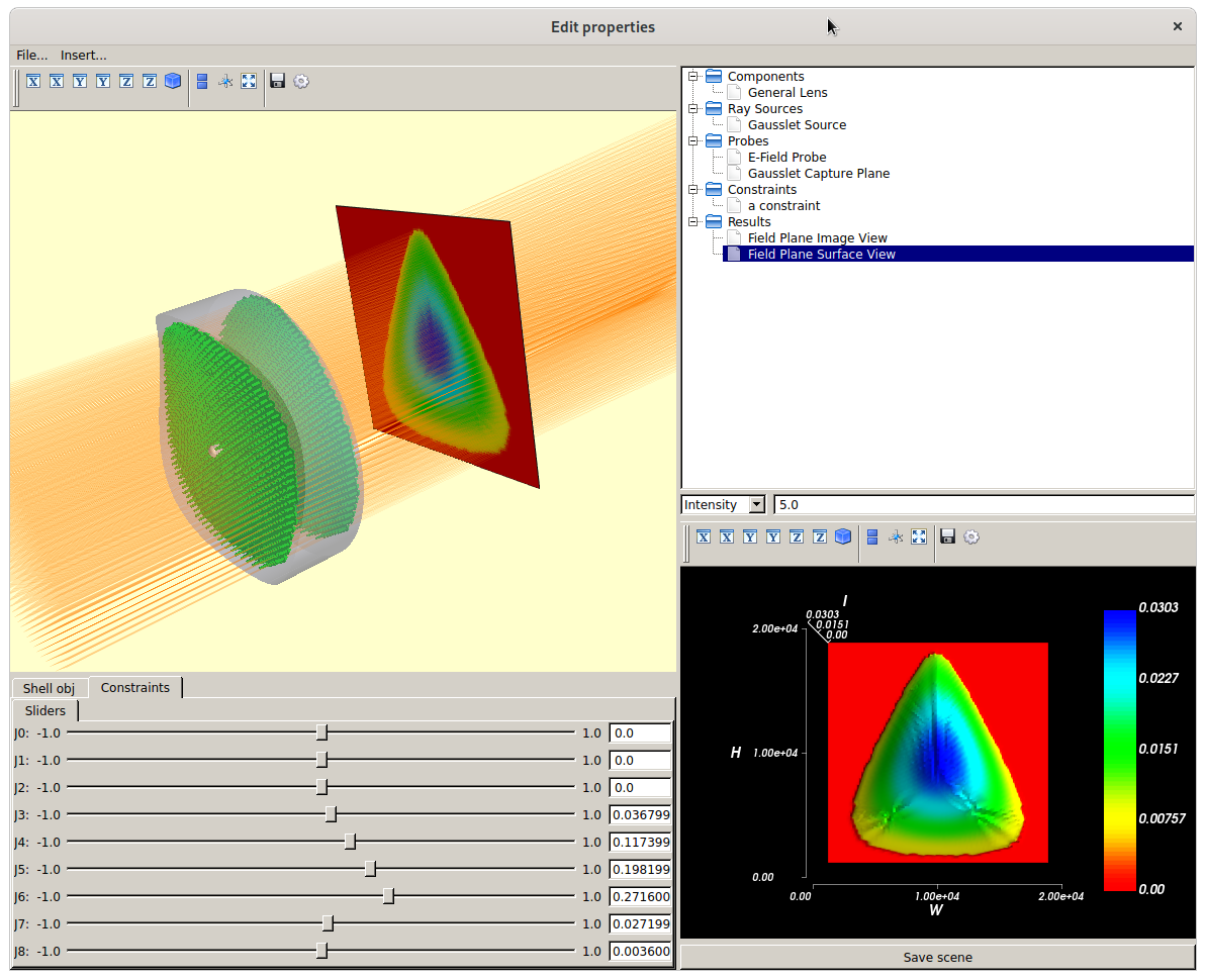
This example also demonstrates the use of a Constraints object to provide some UI controls for easier adjustment of the relevant model parameters.